从基础到进阶详解Python绘制三维图形的全攻略
17人参与 • 2026-04-29 • Python
在数据可视化、科学计算和工程设计领域,三维图形能更直观地呈现数据关系和空间结构。本文将深入讲解 python 中主流的三维绘图库,对比其优缺点,通过实战代码示例帮助大家快速上手,并拓展高级应用场景,让你的数据 “立” 起来!
一、三维绘图库对比
python 生态中有多个成熟的三维绘图库,不同库的设计理念和适用场景差异较大。选择合适的工具,能让绘图效率翻倍。
1. matplotlib
核心定位:python 最基础的绘图库,mplot3d是其扩展的三维模块,适合快速生成简单三维图。
优点:
- 入门门槛低,熟悉 matplotlib 二维绘图的用户可无缝迁移;
- 支持多种三维图形类型(散点图、线图、曲面图等);
- 可与 numpy、pandas 等数据处理库无缝衔接;
- 生成的图形支持高分辨率导出(png、svg、pdf 等)。
缺点:
- 交互性差,默认生成静态图,需额外集成mpl_toolkits.mplot3d的交互工具;
- 绘制复杂场景(如大量数据点、动态效果)时性能较差;
- 对三维模型的细节渲染能力有限(如光照、纹理)。
适用场景:快速生成静态三维数据图表(如科学论文中的数据可视化、简单函数曲面)。
2. plotly
核心定位:交互式可视化库,支持网页端三维图形展示,适合需要动态交互的场景。
优点:
- 交互性极强,支持鼠标拖拽旋转、缩放、hover 显示数据详情;
- 无需额外代码,生成的图形可直接嵌入网页(支持 html 导出);
- 支持复杂三维场景(如 3d 网格图、体积图、三维散点动画);
- 社区文档丰富,示例覆盖多领域。
缺点:
- 静态图导出功能较弱,默认依赖网页渲染;
- 大量数据(如 10 万 + 点)绘制时会出现卡顿;
- 自定义样式(如颜色映射、坐标轴刻度)需学习特定 api。
适用场景:web 端交互式报告、数据 dashboard、动态三维演示。
3. pyvista 与 jupyter notebook 集成
pyvista 是基于 vtk 的高级封装库,旨在简化三维数据可视化流程,同时保留 vtk 的强大功能。
优点:
- 比 mayavi 更简洁的 api,学习曲线平缓
- 与 numpy、pandas 等科学计算库无缝集成
- 出色的 3d 交互体验,支持复杂网格和体数据可视化
- 丰富的过滤和分析工具,适合工程和科学应用
- 良好的 jupyter notebook 支持
缺点:
- 对于简单可视化任务可能显得过于重量级
- 文档相对 plotly 不够完善
- 某些高级功能仍需了解 vtk 概念
二、实战代码示例:从基础到进阶
下面通过 3 个典型场景,演示不同库的三维绘图用法。所有示例均基于 python 3.9+,需提前安装依赖(如pip install matplotlib plotly mayavi numpy)。
示例 1:matplotlib 绘制三维函数曲面
需求:绘制函数
![]()
的曲面图,展示极坐标下的周期性变化。
import numpy as np
import matplotlib.pyplot as plt
from mpl_toolkits.mplot3d import axes3d

# 1. 生成数据
x = np.linspace(-10, 10, 100)  # x轴范围:-10到10,取100个点
y = np.linspace(-10, 10, 100)  # y轴范围:-10到10,取100个点
x, y = np.meshgrid(x, y)       # 生成网格数据(二维数组)
z = np.sin(np.sqrt(x**2 + y**2))  # 计算z值

# 2. 创建三维画布
fig = plt.figure(figsize=(10, 8))  # 设置画布大小
ax = fig.add_subplot(111, projection='3d')  # 创建3d子图

# 3. 绘制曲面图
surf = ax.plot_surface(
    x, y, z,
    cmap='viridis',  # 颜色映射(可选:plasma、coolwarm等)
    alpha=0.8,       # 透明度
    linewidth=0.1    # 网格线宽度
)

# 4. 自定义样式
ax.set_xlabel('x axis', fontsize=12, labelpad=10)  # x轴标签
ax.set_ylabel('y axis', fontsize=12, labelpad=10)  # y轴标签
ax.set_zlabel('z axis', fontsize=12, labelpad=10)  # z轴标签
ax.set_title(r'$z = \sin(\sqrt{x^2 + y^2})$', fontsize=15, pad=20)  # 标题(支持latex)

# 添加颜色条(显示z值与颜色的对应关系)
fig.colorbar(surf, ax=ax, shrink=0.5, aspect=10, label='z value')

# 5. 保存与显示
plt.savefig('3d_surface_matplotlib.png', dpi=300, bbox_inches='tight')  # 高分辨率保存
plt.show()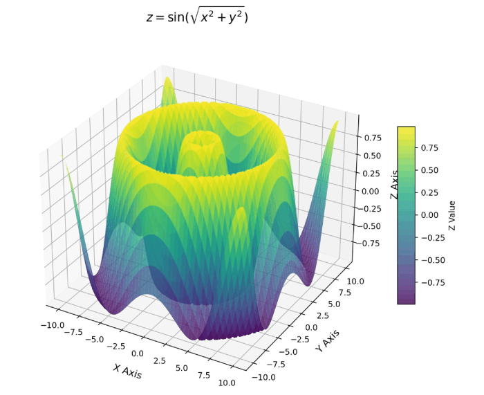
效果说明:生成静态曲面图,颜色随 z 值渐变,可通过鼠标拖动调整视角,但无法在网页中交互。适合插入报告或论文。
示例 2:plotly 绘制交互式三维散点图
需求:模拟 3 组不同类别的数据点(如聚类结果),用三维散点图展示类别分布,支持鼠标交互。
import plotly.graph_objects as go
import numpy as np

# 1. 生成模拟数据(3个类别,每个类别500个点)
np.random.seed(42)  # 固定随机种子,保证结果可复现

# 类别1:均值(0,0,0),标准差0.5
x1 = np.random.normal(0, 0.5, 500)
y1 = np.random.normal(0, 0.5, 500)
z1 = np.random.normal(0, 0.5, 500)

# 类别2:均值(3,3,3),标准差0.5
x2 = np.random.normal(3, 0.5, 500)
y2 = np.random.normal(3, 0.5, 500)
z2 = np.random.normal(3, 0.5, 500)

# 类别3:均值(6,0,3),标准差0.5
x3 = np.random.normal(6, 0.5, 500)
y3 = np.random.normal(0, 0.5, 500)
z3 = np.random.normal(3, 0.5, 500)

# 2. 创建三维散点图
fig = go.figure()

# 添加3个类别的散点
fig.add_trace(go.scatter3d(
    x=x1, y=y1, z=z1,
    mode='markers',  # 标记类型:散点
    marker=dict(
        size=3,        # 点大小
        color='red',   # 颜色
        opacity=0.7    # 透明度
    ),
    name='class 1'  # 图例名称
))

fig.add_trace(go.scatter3d(
    x=x2, y=y2, z=z2,
    mode='markers',
    marker=dict(size=3, color='blue', opacity=0.7),
    name='class 2'
))

fig.add_trace(go.scatter3d(
    x=x3, y=y3, z=z3,
    mode='markers',
    marker=dict(size=3, color='green', opacity=0.7),
    name='class 3'
))

# 3. 自定义布局
fig.update_layout(
    title='3d scatter plot of 3 classes (interactive)',
    title_font=dict(size=16),
    scene=dict(
        xaxis_title='x feature',
        yaxis_title='y feature',
        zaxis_title='z feature',
        xaxis=dict(backgroundcolor='rgba(240,240,240,0.5)'),  # x轴背景色
        yaxis=dict(backgroundcolor='rgba(240,240,240,0.5)'),  # y轴背景色
        zaxis=dict(backgroundcolor='rgba(240,240,240,0.5)')   # z轴背景色
    ),
    legend=dict(
        x=0.1, y=0.9,  # 图例位置
        font=dict(size=12)
    ),
    width=800, height=600  # 图大小
)

# 4. 保存与展示
fig.write_html('3d_scatter_plotly.html')  # 导出为html(支持网页打开)
fig.show()  # 本地展示(默认打开浏览器)
效果说明:打开 html 文件后,可通过鼠标拖拽旋转视角、滚轮缩放,hover 时显示每个点的坐标,点击图例可隐藏 / 显示对应类别。适合 web 端分享或动态演示。
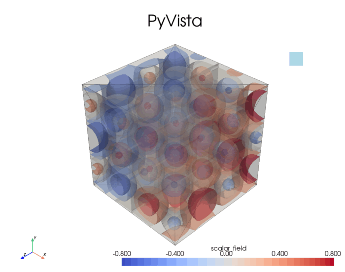
案例 3:使用 pyvista 可视化复杂三维网格和体数据
pyvista 特别擅长处理三维网格数据和体数据,下面示例展示如何创建并可视化一个复杂的三维结构:
import pyvista as pv
import numpy as np

# 确保中文显示正常
pv.set_plot_theme("document")

# 1. 创建一个复杂的三维网格 - 带孔的立方体
# 创建一个基础立方体
cube = pv.cube(x_length=2, y_length=2, z_length=2)
# 对立方体进行三角形化处理,使用更精细的参数
cube = cube.triangulate(progress_bar=false)

# 在立方体上打几个孔
spheres = [
    pv.sphere(radius=0.5, center=(0.5, 0, 0)),
    pv.sphere(radius=0.5, center=(-0.5, 0, 0)),
    pv.sphere(radius=0.5, center=(0, 0.5, 0)),
    pv.sphere(radius=0.5, center=(0, -0.5, 0))
]

# 布尔运算:从立方体中减去球体(创建孔洞)
tolerance = 1e-6  # 设置容差
for sphere in spheres:
    # 对球体进行更彻底的三角形化
    sphere = sphere.triangulate(progress_bar=false)
    # 确保网格质量
    if not sphere.is_all_triangles:
        sphere = sphere.triangulate(progress_bar=false)

    # 执行布尔运算时指定容差
    cube = cube.boolean_difference(
        sphere,
        tolerance=tolerance,
        progress_bar=false
    )

    # 确保结果是三角形网格
    if not cube.is_all_triangles:
        cube = cube.triangulate(progress_bar=false)

    # 检查是否有有效数据
    if cube.n_points == 0 or cube.n_cells == 0:
        print("警告:布尔运算后网格为空,调整容差或几何参数")
        # 适当增大容差重试
        tolerance *= 2
        # 重新创建立方体以避免累积错误
        cube = pv.cube(x_length=2, y_length=2, z_length=2).triangulate()

# 2. 创建体数据 - 立方体内部的标量场
# 生成网格点
x = np.linspace(-1, 1, 50)
y = np.linspace(-1, 1, 50)
z = np.linspace(-1, 1, 50)
grid = pv.rectilineargrid(x, y, z)

# 在网格上创建一个复杂的标量场
xx, yy, zz = grid.points.t
scalar_field = np.sin(5 * xx) * np.cos(5 * yy) * np.sin(5 * zz) + 0.5 * xx

# 将标量场添加到网格
grid["scalar_field"] = scalar_field

# 3. 创建可视化场景
p = pv.plotter(notebook=false, window_size=[1000, 800])

# 添加立方体网格
p.add_mesh(
    cube,
    color="white",
    show_edges=true,
    edge_color="black",
    opacity=0.3,
    label="带孔立方体"
)

# 添加体数据的等值面
contours = grid.contour([-0.8, -0.4, 0, 0.4, 0.8])
p.add_mesh(
    contours,
    cmap="coolwarm",
    opacity=0.8,
    label="标量场等值面"
)

# 添加坐标轴和标题
p.add_axes()
p.add_title("pyvista三维网格与体数据可视化")
p.add_legend()

# 设置相机位置
p.camera_position = [
    (5, 5, 5),  # 相机位置
    (0, 0, 0),  # 焦点
    (0, 1, 0)  # 上方向
]

# 显示场景
p.show()

# 4. 进阶:创建交互式切片
p = pv.plotter(notebook=false, window_size=[1000, 800])
p.add_mesh(grid.contour([0]), cmap="coolwarm", label="标量场等值面")

# 添加可交互的切片平面
p.add_slice(grid, normal="x", show_edges=true)
p.add_slice(grid, normal="y", show_edges=true)

p.add_axes()
p.add_title("交互式体数据切片")
p.add_legend()
p.show()
总结
选择合适的三维绘图库应根据具体需求:
- 快速原型设计和简单可视化:优先选择 matplotlib,学习成本低,集成方便
- 交互式展示和网页分享:选择 plotly,其生成的交互式图表体验最佳
- 科学计算和工程应用:选择 pyvista,它提供了强大的三维网格和体数据处理能力,api 友好,同时保留了 vtk 的强大功能,适合处理复杂的科学和工程数据。
三维可视化是探索数据空间特征的强大工具,通过本文介绍的方法和技巧,你可以根据项目需求选择合适的工具,创建既美观又有信息量的三维图形。
以上就是从基础到进阶详解python绘制三维图形的全攻略的详细内容,更多关于python绘制三维图形的资料请关注代码网其它相关文章!
赞 (0)
您想发表意见!!点此发布评论


发表评论