机器学习——逻辑回归_机器学习

一. 逻辑回归（logistic regression）

二. 逻辑回归模型的算法原理

1. 处理数据

2. 引入sigmoid函数

一. 逻辑回归（logistic regression）

逻辑回归是一个非常经典的解决分类问题的机器学习方法，该算法的主要思想是将输入变量的线性组合映射到0到1之间的概率，用于预测二元输出变量。

二. 逻辑回归模型的算法原理

1. 处理数据

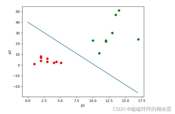
假设我们有一个二分类问题，需要预测一个样本属于两个类别中的哪一个。

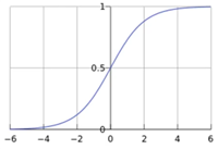
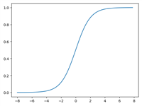
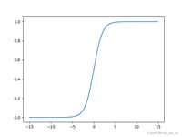
2. 引入sigmoid函数

1）公式： $g(z)=\frac{1}{1+e^{-z}}$

2）sigmoid图像：

$y_{i}$

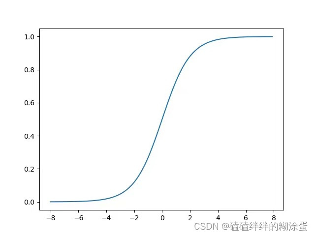
注：将线性回归的结果映射到[0,1]区间上，实质上就是完成了二分类任务。

3. 引入梯度下降法

梯度下降法通过反复迭代来最小化损失函数，直至找到最优解，起到了优化模型参数、寻找最优解、调节学习率和处理大规模数据的作用。是逻辑回归模型中常用的优化算法之一，能够有效地提升模型的性能。

其中，损失函数公式为： $j(w)=-\frac{1}{n}\sum_{i=1}^{n}y_{i}log(z_{i})+(1-y_{i})log(1-g(z_{i}))$ ， $z_{i}$ 是第i个样本的线性组合， $y_{i}$ 是对应的类别标签（0或1）。

三. 逻辑回归与线性回归的相同点和不同点

1）相同点：

逻辑回归与线性回归都是一种广义线性模型（generalized linear model）。

2）不同点：

1）逻辑回归假设因变量 y 服从伯努利分布，而线性回归假设因变量 y 服从高斯分布。

2）逻辑回归用于分类问题，线性回归用于拟合回归问题。

注：逻辑回归算法去除sigmoid映射函数就是一个线性回归。也就是说，逻辑回归以线性回归为理论支持，并通过sigmoid函数引入了非线性因素，可以轻松处理0/1分类问题。

四. 算法实现

1. 导入包

import numpy as np
import matplotlib.pyplot as plt
from sklearn.datasets import load_iris
from sklearn.model_selection import train_test_split

2. 定义随机数种子

# 设置随机种子
seed_value = 2023
np.random.seed(seed_value)

3. 定义逻辑回归模型

3.1 初始化模型

# 初始化参数
self.weights = np.random.randn(x.shape[1])
self.bias = 0

3.2 正向传播

# 计算sigmoid函数的预测值, y_hat = sigmoid(w * x + b)
y_hat = sigmoid(np.dot(x, self.weights) + self.bias)

3.3 损失函数

# 计算损失函数
loss = (-1 / len(x)) * np.sum(y * np.log(y_hat) + (1 - y) * np.log(1 - y_hat))

3.4 反向传播

# 计算梯度
dw = (1 / len(x)) * np.dot(x.t, (y_hat - y))
db = (1 / len(x)) * np.sum(y_hat - y)

# 更新参数
self.weights -= self.learning_rate * dw
self.bias -= self.learning_rate * db

3.5 模型预测

# 预测
def predict(self, x):
    y_hat = sigmoid(np.dot(x, self.weights) + self.bias)
    y_hat[y_hat >= 0.5] = 1
    y_hat[y_hat < 0.5] = 0
    return y_hat

3.6 模型精度

# 精度
def score(self, y_pred, y):
    accuracy = (y_pred == y).sum() / len(y)
    return accuracy

3.7 用鸢尾花数据集来预测模型

import numpy as np
import matplotlib.pyplot as plt
from sklearn.datasets import load_iris
from sklearn.model_selection import train_test_split

# 设置随机种子
seed_value = 2023
np.random.seed(seed_value)

# sigmoid激活函数
def sigmoid(z):
    return 1 / (1 + np.exp(-z))

# 定义逻辑回归算法
class logisticregression:
    def __init__(self, learning_rate=0.003, iterations=100):
        self.learning_rate = learning_rate # 学习率
        self.iterations = iterations # 迭代次数

    def fit(self, x, y):
        # 初始化参数
        self.weights = np.random.randn(x.shape[1])
        self.bias = 0

        # 梯度下降
        for i in range(self.iterations):
            # 计算sigmoid函数的预测值, y_hat = w * x + b
            y_hat = sigmoid(np.dot(x, self.weights) + self.bias)

            # 计算损失函数
            loss = (-1 / len(x)) * np.sum(y * np.log(y_hat) + (1 - y) * np.log(1 - y_hat))

            # 计算梯度
            dw = (1 / len(x)) * np.dot(x.t, (y_hat - y))
            db = (1 / len(x)) * np.sum(y_hat - y)

            # 更新参数
            self.weights -= self.learning_rate * dw
            self.bias -= self.learning_rate * db

            # 打印损失函数值
            if i % 10 == 0:
                print(f"loss after iteration {i}: {loss}")

    # 预测
    def predict(self, x):
        y_hat = sigmoid(np.dot(x, self.weights) + self.bias)
        y_hat[y_hat >= 0.5] = 1
        y_hat[y_hat < 0.5] = 0
        return y_hat
    
    # 精度
    def score(self, y_pred, y):
        accuracy = (y_pred == y).sum() / len(y)
        return accuracy

# 导入数据
iris = load_iris()
x = iris.data[:, :2]
y = (iris.target != 0) * 1

# 划分训练集、测试集
x_train, x_test, y_train, y_test = train_test_split(x, y, test_size=0.15, random_state=seed_value)

# 训练模型
model = logisticregression(learning_rate=0.03, iterations=1000)
model.fit(x_train, y_train)

# 结果
y_train_pred = model.predict(x_train)
y_test_pred = model.predict(x_test)

score_train = model.score(y_train_pred, y_train)
score_test = model.score(y_test_pred, y_test)

print('训练集accuracy: ', score_train)
print('测试集accuracy: ', score_test)

# 可视化决策边界
x1_min, x1_max = x[:, 0].min() - 0.5, x[:, 0].max() + 0.5
x2_min, x2_max = x[:, 1].min() - 0.5, x[:, 1].max() + 0.5
xx1, xx2 = np.meshgrid(np.linspace(x1_min, x1_max, 100), np.linspace(x2_min, x2_max, 100))
z = model.predict(np.c_[xx1.ravel(), xx2.ravel()])
z = z.reshape(xx1.shape)
plt.contourf(xx1, xx2, z, cmap=plt.cm.spectral)
plt.scatter(x[:, 0], x[:, 1], c=y, cmap=plt.cm.spectral)
plt.xlabel("sepal length")
plt.ylabel("sepal width")
plt.show()