《机器学习实战》——第3章 决策树

3.1 决策树的构造

优点：计算复杂度不高，输出结果易于理解，对中间值的缺失不敏感，可以处理不相关特征数据。
缺点：可能会产生过度匹配的问题。
适用数据类型：数值型和标称型。

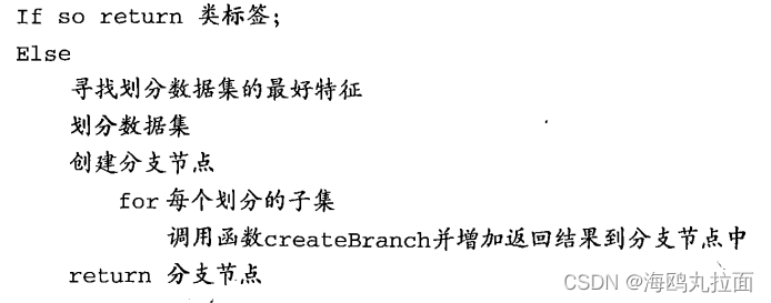
创建分支的伪代码函数 createbranch() 如下所示：

3.1.1 信息增益

划分数据集的大原则是：将无序的数据变得更加有序。划分数据集之前之后信息发生的变化称为信息增益。在可以评测哪种数据划分方式是最好的数据划分之前，我们必须学习如何计算信息增益。

如果待分类的事物可能划分在多个分类之中，则符号xi的信息定义为：

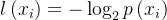
其中p(xi)是选择该分类的概率。

计算所有类别所有可能值包含的信息期望值：

其中n是分类的数目。

创建trees.py文件，计算给定数据集的熵：

import math import log
def calcshannonent(dataset):
    numentries = len(dataset)
    labelcounts = {}
    for featvec in dataset: #the the number of unique elements and their occurance
        currentlabel = featvec[-1]
        if currentlabel not in labelcounts.keys(): labelcounts[currentlabel] = 0
        labelcounts[currentlabel] += 1
    shannonent = 0.0
    for key in labelcounts:
        prob = float(labelcounts[key])/numentries
        shannonent -= prob * log(prob,2) #log base 2
    return shannonent

1. 计算数据集中实例的总数。我们也可以在需要时再计算这个值，但是由于代码中多次用到这个值，为了提高代码效率，我们显式地声明一个变量保存实例总数。
2. 创建一个数据字典，它的键值是最后-列的数值.如果当前键值不存在，则扩展字典并将当前键值加人字典。每个键值都记录了当前类别出现的次数。
3. 使用所有类标签的发生频率计算类别出现的概率。我们将用这个概率计算香农嫡，统计所有类标签发生的次数。下面我们看看如何使用嫡划分数据集。

创建一个自己的 createdataset() 函数：

def createdataset():
    dataset = [[1, 1, 'yes'],
               [1, 1, 'yes'],
               [1, 0, 'no'],
               [0, 1, 'no'],
               [0, 1, 'no']]
    labels = ['no surfacing','flippers']
    return dataset, labels

测试函数效果：

import trees

mydat,labels = trees.createdataset()
test1 = trees.calcshannonent(mydat)
print(mydat)
print(test1)

熵越高，则混合的数据也越多。

import trees

mydat,labels = trees.createdataset()
mydat[0][-1] = 'maybe'
test1 = trees.calcshannonent(mydat)
print(mydat)
print(test1)

3.1.2 划分数据集

分类算法除了需要测量信息嫡，还需要划分数据集，度量花费数据集的嫡，以便判断当前是否正确地划分了数据集。我们将对每个特征划分数据集的结果计算一次信息嫡，然后判断按照哪个特征划分数据集是最好的划分方式。

为trees.py添加代码：

def splitdataset(dataset, axis, value):
    retdataset = []
    for featvec in dataset:
        if featvec[axis] == value:
            reducedfeatvec = featvec[:axis]     #chop out axis used for splitting
            reducedfeatvec.extend(featvec[axis+1:])
            retdataset.append(reducedfeatvec)
    return retdataset

代码使用了三个输入参数:待划分的数据集、划分数据集的特征、特征的返回值。需要注意的是，python语言不用考虑内存分配问题。python语言在函数中传递的是列表的引用，在函数内部对列表对象的修改，将会影响该列表对象的整个生存周期。为了消除这个不良影响,我们需要在函数的开始声明一个新列表对象。因为该函数代码在同一数据集上被调用多次，为了不修改原始数据集，创建一个新的列表对象。数据集这个列表中的各个元素也是列表，我们要遍历数据集中的每个元素，一旦发现符合要求的值，则将其添加到新创建的列表中。在if语句中，程序将符合特征的数据抽取出来。后面讲述得更简单，这里我们可以这样理解这段代码:当我们按照某个特征划分数据集时，就需要将所有符合要求的元素抽取出来。代码中使用了python语言列表类型自带的extend()和append ()方法。这两个方法功能类似，但是在处理多个列表时，这两个方法的处理结果是完全不同的。

测试函数 splitdataset()：

import trees
mydat,labels = trees.createdataset()
print(mydat)
test1 = trees.splitdataset(mydat,0,1)
test2 = trees.splitdataset(mydat,0,0)
print(test1)
print(test2)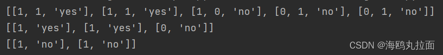

为trees.py添加下面的代码：

def choosebestfeaturetosplit(dataset):
    numfeatures = len(dataset[0]) - 1      #the last column is used for the labels
    baseentropy = calcshannonent(dataset)
    bestinfogain = 0.0; bestfeature = -1
    for i in range(numfeatures):        #iterate over all the features
        featlist = [example[i] for example in dataset]#create a list of all the examples of this feature
        uniquevals = set(featlist)       #get a set of unique values
        newentropy = 0.0
        for value in uniquevals:
            subdataset = splitdataset(dataset, i, value)
            prob = len(subdataset)/float(len(dataset))
            newentropy += prob * calcshannonent(subdataset)     
        infogain = baseentropy - newentropy     #calculate the info gain; ie reduction in entropy
        if (infogain > bestinfogain):       #compare this to the best gain so far
            bestinfogain = infogain         #if better than current best, set to best
            bestfeature = i
    return bestfeature                      #returns an integer

该函数实现选取特征，划分数据集，计算得出最好的划分数据集的特征。 

在开始划分数据集之前，第3行代码计算了整个数据集的原始香农嫡，我们保存最初的无序度量值，用于与划分完之后的数据集计算的嫡值进行比较。第1个for循环遍历数据集中的所有特征。使用列表推导(list comprehension)来创建新的列表，将数据集中所有第i个特征值或者所有可能存在的值写人这个新list中。然后使用python语言原生的集合(set)数据类型。集合数据类型与列表类型相似，不同之处仅在于集合类型中的每个值互不相同。从列表中创建集合是python语言得到列表中唯一元素值的最快方法。

遍历当前特征中的所有唯一属性值，对每个特征划分一次数据集，然后计算数据集的新熵值，并对所有唯一特征值得到的熵求和。信息增益是熵的减少或者是数据无序度的减少，大家肯定对于将熵用于度量数据无序度的减少更容易理解。最后，比较所有特征中的信息增益，返回最好特征划分的索引值。

import trees
mydat,labels = trees.createdataset()
trees.choosebestfeaturetosplit(mydat)
print(mydat)

3.1.3 递归构建决策树

从数据集构造决策树算法所需子功能模块工作原理：得到原始数据集，基于最好的属性值划分数据集，由于特征值可能多于两个，因此可能存在大于两个分支的数据集划分。第一次划分后，数据将被向下传递到树分支的下一个节点，在这个节点上，我们可以再次划分数据。因此我们可以采用递归的原则处理数据集。

递归结束条件：程序遍历完所有划分数据集的属性，或者每个分支下的所有实例都具有相同的分类。如果所有实例具有相同的分类，则得到一个叶子节点或者终止块。任何到达叶子节点的数据必然属于叶子节点的分类。

添加下面的代码到trees.py中：

import operator
def majoritycnt(classlist):
    classcount={}
    for vote in classlist:
        if vote not in classcount.keys(): classcount[vote] = 0
        classcount[vote] += 1
    sortedclasscount = sorted(classcount.iteritems(), key=operator.itemgetter(1), reverse=true)
    return sortedclasscount[0][0]

该函数使用分类名称的列表，创建键值为classlist中唯一值的数据字典，字典对象存储了classlist中每个类标签出现的频率，最后利用operator操作键值排序字典，并返回出现次数最多的分类名称。

def createtree(dataset,labels):
    classlist = [example[-1] for example in dataset]
    if classlist.count(classlist[0]) == len(classlist): 
        return classlist[0]#stop splitting when all of the classes are equal
    if len(dataset[0]) == 1: #stop splitting when there are no more features in dataset
        return majoritycnt(classlist)
    bestfeat = choosebestfeaturetosplit(dataset)
    bestfeatlabel = labels[bestfeat]
    mytree = {bestfeatlabel:{}}
    del(labels[bestfeat])
    featvalues = [example[bestfeat] for example in dataset]
    uniquevals = set(featvalues)
    for value in uniquevals:
        sublabels = labels[:]       #copy all of labels, so trees don't mess up existing labels
        mytree[bestfeatlabel][value] = createtree(splitdataset(dataset, bestfeat, value),sublabels)
    return mytree

代码使用两个输入参数:数据集和标签列表。标签列表包含了数据集中所有特征的标签，算法本身并不需要这个变量，但是为了给出数据明确的含义，我们将它作为一个输入参数提供。此外，前面提到的对数据集的要求这里依然需要满足。上述代码首先创建了名为classlist的列表变量,其中包含了数据集的所有类标签。递归函数的第一个停止条件是所有的类标签完全相同，则直接返回该类标签。递归函数的第二个停止条件是使用完了所有特征，仍然不能将数据集划分成仅包含唯一类别的分组。由于第二个条件无法简单地返回唯一的类标签，这里使用之前的函数挑选出现次数最多的类别作为返回值。
下一步程序开始创建树，这里使用python语言的字典类型存储树的信息，当然也可以声明特殊的数据类型存储树，但是这里完全没有必要。字典变量mytree存储了树的所有信息，这对于其后绘制树形图非常重要。当前数据集选取的最好特征存储在变量bestfeat中，得到列表包含的所有属性值。
最后代码遍历当前选择特征包含的所有属性值，在每个数据集划分上递归调用函数createtree()，得到的返回值将被插入到字典变量mytree中，因此函数终止执行时，字典中将会嵌套很多代表叶子节点信息的字典数据。在解释这个嵌套数据之前，我们先看-一下循环的第一行sublabels = labels[ : ]，这行代码复制了类标签，并将其存储在新列表变量sublabels中。之所以这样做，是因为在python语言中函数参数是列表类型时，参数是按照引用方式传递的。为了保证每次调用函数createtree()时不改变原始列表的内容，使用新变量sublabels代替原始列表。

测试代码的输出结果：

import trees
mydat,labels = trees.createdataset()
mytree = trees.createtree(mydat,labels)
print(mytree)

变量mytree包含了很多代表树结构信息的嵌套字典，从左边开始，第一个关键字no surfacing是第一个划分数据集的特征名称，该关键字的值也是另一个数据字典。第二个关键字是no surfacing特征划分的数据集，这些关键字的值是no surfacing节点的子节点。这些值可能是类标签，也可能是另一个数据字典。如果值是类标签，则该子节点是叶子节点;如果值是另一个数据字典，则子节点是一个判断节点，这种格式结构不断重复就构成了整棵树。

3.2 在python中使用matplotlib注解绘制树形图

3.2.1 matplotlib注解

annotations是matplotlib提供的一个注解工具，能够在数据图形上添加文本注释。创建 treeplotter.py 文件，添加下列代码：

import matplotlib.pyplot as plt
decisionnode = dict(boxstyle="sawtooth", fc="0.8")
leafnode = dict(boxstyle="round4", fc="0.8")
arrow_args = dict(arrowstyle="<-")

def plotnode(nodetxt, centerpt, parentpt, nodetype):
    createplot.ax1.annotate(nodetxt, xy=parentpt,  xycoords='axes fraction',
             xytext=centerpt, textcoords='axes fraction',
             va="center", ha="center", bbox=nodetype, arrowprops=arrow_args)
    
def createplot():
    fig = plt.figure(1, facecolor='white')
    fig.clf()
    createplot.ax1 = plt.subplot(111, frameon=false) #ticks for demo puropses 
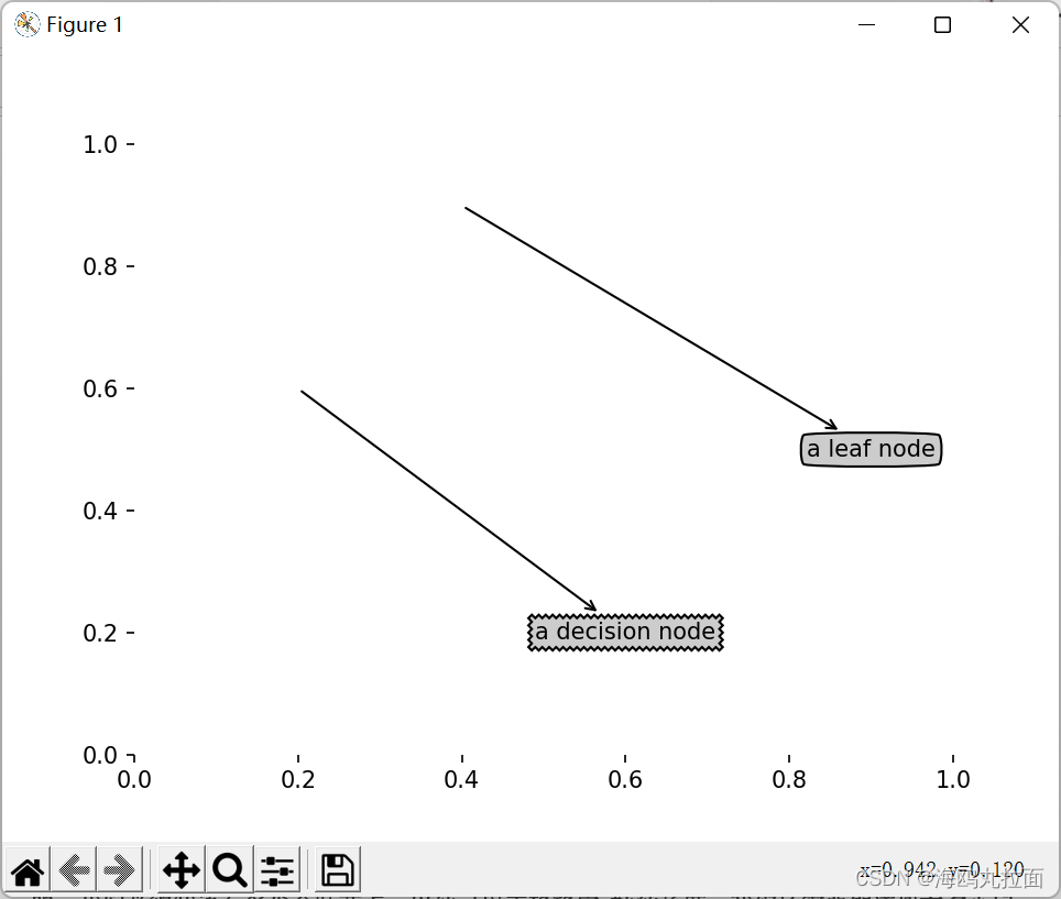
    plotnode('a decision node', (0.5, 0.1), (0.1, 0.5), decisionnode)
    plotnode('a leaf node', (0.8, 0.1), (0.3, 0.8), leafnode)
    plt.show()

代码定义了树节点格式的常量。然后定义plotnode( )函数执行了实际的绘图功能，该函数需要一个绘图区，该区域由全局变量createplot.ax1定义。python语言中所有的变量默认都是全局有效的，只要我们清楚知道当前代码的主要功能，并不会引入太大的麻烦。最后定义createplot ()函数，它是这段代码的核心。createplot ( )函数首先创建了一个新图形并清空绘图区，然后在绘图区上绘制两个代表不同类型的树节点，后面我们将用这两个节点绘制树形图。

测试函数的输出结果：

import treeplotter
treeplotter.createplot()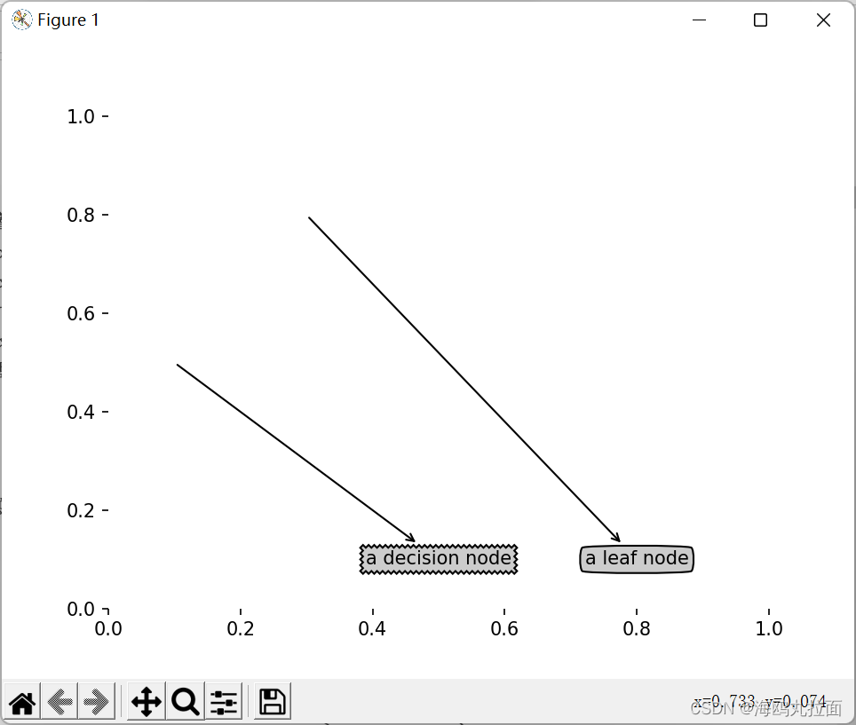

改变函数plotnode()可以得到不同的曲线。

3.2.2 构造注解树

添加两个函数到文件中，以获取叶节点的数目和树的层数：

def getnumleafs(mytree):
    numleafs = 0
    firststr = mytree.keys()[0]
    seconddict = mytree[firststr]
    for key in seconddict.keys():
        if type(seconddict[key]).__name__=='dict':#test to see if the nodes are dictonaires, if not they are leaf nodes
            numleafs += getnumleafs(seconddict[key])
        else:   numleafs +=1
    return numleafs

def gettreedepth(mytree):
    maxdepth = 0
    firststr = mytree.keys()[0]
    seconddict = mytree[firststr]
    for key in seconddict.keys():
        if type(seconddict[key]).__name__=='dict':#test to see if the nodes are dictonaires, if not they are leaf nodes
            thisdepth = 1 + gettreedepth(seconddict[key])
        else:   thisdepth = 1
        if thisdepth > maxdepth: maxdepth = thisdepth
    return maxdepth

上述程序中的两个函数具有相同的结构,。这里使用的数据结构说明了如何在python字典类型中存储树信息。第一个关键字是第一次划分数据集的类别标签，附带的数值表示子节点的取值。从第一个关键字出发，我们可以遍历整棵树的所有子节点。使用python提供的type ( )函数可以判断子节点是否为字典类型。如果子节点是字典类型，则该节点也是一个判断节点，需要递归调用getnumleafs ( )函数。getnumleafs ( )函数遍历整棵树，累计叶子节点的个数，并返回该数值。第2个函数gettreedepth( )计算遍历过程中遇到判断节点的个数。该函数的终止条件是叶子节点，一旦到达叶子节点，则从递归调用中返回，并将计算树深度的变量加一。为了节省时间，函数retrievetree输出预先存储的树信息，避免了每次测试代码时都要从数据中创建树的麻烦。

添加下面的代码到文件中：

def retrievetree(i):
    listoftrees =[{'no surfacing': {0: 'no', 1: {'flippers': {0: 'no', 1: 'yes'}}}},
                  {'no surfacing': {0: 'no', 1: {'flippers': {0: {'head': {0: 'no', 1: 'yes'}}, 1: 'no'}}}}
                  ]
    return listoftrees[i]

import treeplotter
test1 = treeplotter.retrievetree(1)
mytree = treeplotter.retrievetree(0)
test2 = treeplotter.getnumleafs(mytree)
test3 = treeplotter.gettreedepth(mytree)
print(test1)
print(test2)
print(test3)

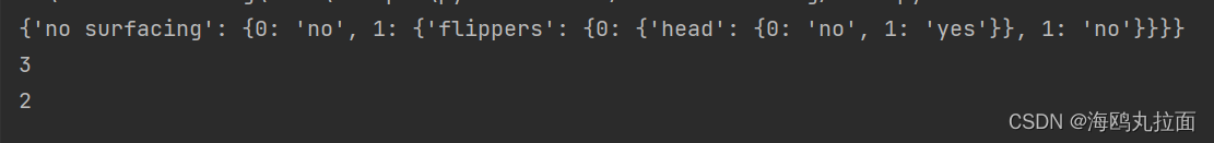
函数retrievepree()主要用于测试,返回预定义的树结构。上述命令中调用getnumleafs ()函数返回值为3，等于树0的叶子节点数;调用gettreedepths()函数也能够正确返回树的层数。

添加下面代码到文件中，同时对前文定义的createplot（）进行更新：

def plotmidtext(cntrpt, parentpt, txtstring):
    xmid = (parentpt[0]-cntrpt[0])/2.0 + cntrpt[0]
    ymid = (parentpt[1]-cntrpt[1])/2.0 + cntrpt[1]
    createplot.ax1.text(xmid, ymid, txtstring, va="center", ha="center", rotation=30)

def plottree(mytree, parentpt, nodetxt):#if the first key tells you what feat was split on
    numleafs = getnumleafs(mytree)  #this determines the x width of this tree
    depth = gettreedepth(mytree)
    firststr = mytree.keys()[0]     #the text label for this node should be this
    cntrpt = (plottree.xoff + (1.0 + float(numleafs))/2.0/plottree.totalw, plottree.yoff)
    plotmidtext(cntrpt, parentpt, nodetxt)
    plotnode(firststr, cntrpt, parentpt, decisionnode)
    seconddict = mytree[firststr]
    plottree.yoff = plottree.yoff - 1.0/plottree.totald
    for key in seconddict.keys():
        if type(seconddict[key]).__name__=='dict':#test to see if the nodes are dictonaires, if not they are leaf nodes   
            plottree(seconddict[key],cntrpt,str(key))        #recursion
        else:   #it's a leaf node print the leaf node
            plottree.xoff = plottree.xoff + 1.0/plottree.totalw
            plotnode(seconddict[key], (plottree.xoff, plottree.yoff), cntrpt, leafnode)
            plotmidtext((plottree.xoff, plottree.yoff), cntrpt, str(key))
    plottree.yoff = plottree.yoff + 1.0/plottree.totald

def createplot(intree):
    fig = plt.figure(1, facecolor='white')
    fig.clf()
    axprops = dict(xticks=[], yticks=[])
    createplot.ax1 = plt.subplot(111, frameon=false, **axprops)    #no ticks
    #createplot.ax1 = plt.subplot(111, frameon=false) #ticks for demo puropses 
    plottree.totalw = float(getnumleafs(intree))
    plottree.totald = float(gettreedepth(intree))
    plottree.xoff = -0.5/plottree.totalw; plottree.yoff = 1.0;
    plottree(intree, (0.5,1.0), '')
    plt.show()

函数createplot ()是我们使用的主函数，它调用了plottree( )，函数plottree又依次调用了前面介绍的函数和plotmidtext()。绘制树形图的很多工作都是在函数plottree ( )中完成的，函数plottree( )首先计算树的宽和高。全局变量plottree.totalw存储树的宽度，全局变量plottree.totald存储树的深度，我们使用这两个变量计算树节点的摆放位置，这样可以将树绘制在水平方向和垂直方向的中心位置。与函数getnumleafs()和gettreedepth()类似，函数plottree( )也是个递归函数。树的宽度用于计算放置判断节点的位置，主要的计算原则是将它放在所有叶子节点的中间，而不仅仅是它子节点的中间。同时我们使用两个全局变量plottree.xoff和plottree.yoff追踪已经绘制的节点位置，以及放置下一个节点的恰当位置。另一个需要说明的问题是，绘制图形的x轴有效范围是0.0到1.0，y轴有效范围也是0.0~1.0。为了方便起见，图3-6给出具体坐标值，实际输出的图形中并没有x、y坐标。通过计算树包含的所有叶子节点数，划分图形的宽度，从而计算得到当前节点的中心位置，也就是说，我们按照叶子节点的数目将x轴划分为若干部分。按照图形比例绘制树形图的最大好处是无需关心实际输出图形的大小，旦图形大小发生了变化，函数会自动按照图形大小重新绘制。如果以像素为单位绘制图形，则缩放图形就不是一件简单的工作。
接着，绘出子节点具有的特征值，或者沿此分支向下的数据实例必须具有的特征值③。使用函数plotmidtext( )计算父节点和子节点的中间位置，并在此处添加简单的文本标签信息r。
然后，按比例减少全局变量plottree.yoff，并标注此处将要绘制子节点④，这些节点即可以是叶子节点也可以是判断节点，此处需要只保存绘制图形的轨迹。因为我们是自顶向下绘制图形，因此需要依次递减y坐标值，而不是递增y坐标值。然后程序采用函数getnumleafs()和gettreodepth()以相同的方式递归遍历整棵树，如果节点是叶子节点则在图形上画出叶子节点，如果不是叶子节点则递归调用plottree()函数。在绘制了所有子节点之后，增加全局变量y的偏移。

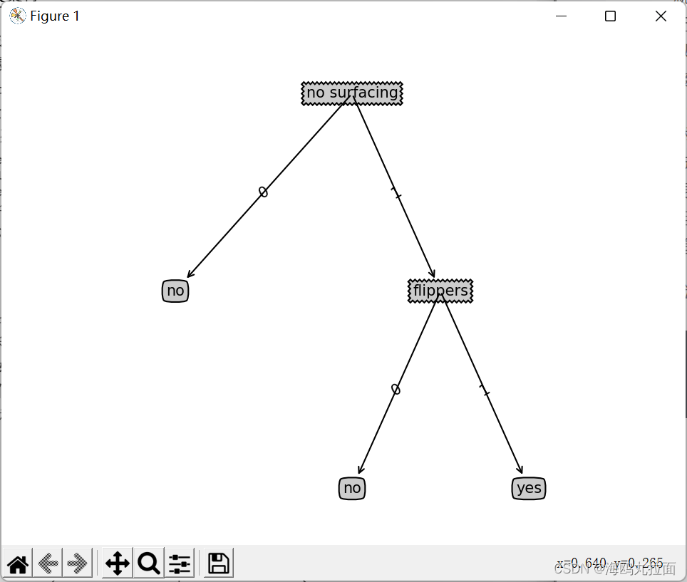
验证输出效果：

import treeplotter
mytree = treeplotter.retrievetree(0)
treeplotter.createplot(mytree)

3.3 测试和存储分类器

3.3.1 测试算法：使用决策树执行分类

依靠训练数据构造了决策树之后，我们可以将它用于实际数据的分类。在执行数据分类时，需要决策树以及用于构造树的标签向量。然后，程序比较测试数据与决策树上的数值，递归执行该过程直到进人叶子节点;最后将测试数据定义为叶子节点所属的类型。

添加下面的代码到trees.py中：

def classify(inputtree,featlabels,testvec):
    firststr = list(inputtree.keys())[0]
    seconddict = inputtree[firststr]
    featindex = featlabels.index(firststr)
    key = testvec[featindex]
    valueoffeat = seconddict[key]
    if isinstance(valueoffeat, dict): 
        classlabel = classify(valueoffeat, featlabels, testvec)
    else: classlabel = valueoffeat
    return classlabel

该函数也是一个递归函数，在存储带有特征的数据会面临一个问题：程序无法确定特征在数据集中的位置，例如前面例子的第一个用于划分数据集的特征是nosurfacing属性,但是在实际数据集中该属性存储在哪个位置?是第一个属性还是第二个属性?特征标签列表将帮助程序处理这个问题。使用index方法查找当前列表中第一个匹配firststr变量的元素。然后代码递归遍历整棵树，比较testvec变量中的值与树节点的值，如果到达叶子节点，则返回当前节点的分类标签。

import treeplotter
import trees
mydat,labels = trees.createdataset()
mytree = treeplotter.retrievetree(0)
test1 = trees.classify(mytree,labels,[1,0])
test2 = trees.classify(mytree,labels,[1,1])
print(labels)
print(test1)
print(test2)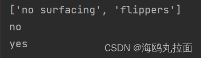

两个节点：名字为0的叶子节点，类标签为no；名为flippers的判断节点，此处进入递归调用，flippers节点有两个子节点。

3.3.2 使用算法：决策树的存储

构造决策树十分耗时，但用创建好的决策树解决分类问题则可以很快完成。将下面的代码加入trees.py：

def storetree(inputtree, filename):
    import pickle
    fw = open(filename, 'w')
    pickle.dump(inputtree, fw)
    fw.close()

def grabtree(filename):
    import pickle
    fr = open(filename)
    return pickle.load(fr)

测试效果：

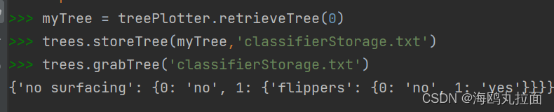
我们将分类器存储在硬盘上，不用每次对数据分类时重新学习以便，这也是决策树的优点之一。

3.4 示例：使用决策树预测隐形眼镜类型

通过下面的代码加载数据：

import treeplotter
import trees
fr = open('lenses.txt')
lenses= [inst.strip().split('\t') for inst in fr.readlines()]
lenseslabels= ['age', 'prescript ' , 'astigmatic', 'tearrate']
lensestree = trees.createtree(lenses , lenseslabels)
print(lensestree)
treeplotter.createplot(lensestree)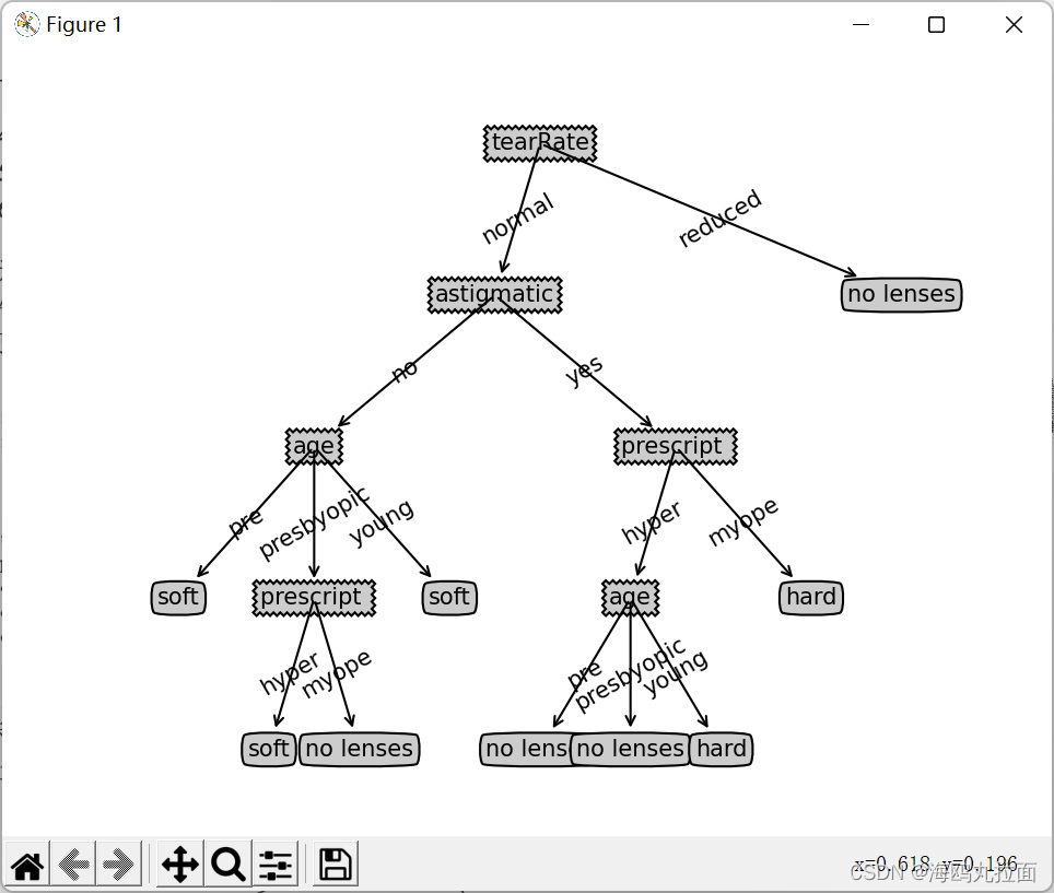

文本难以分辨决策树的结构，最后一行代码调用了函数绘制树形图。

3.5 本章小结

决策树分类器就像带有终止块的流程图，终止块表示分类结果。开始处理数据集时，我们首先需要测量集合中数据的不一致性，也就是嫡，然后寻找最优方案划分数据集，直到数据集中的所有数据属于同一分类。id3算法可以用于划分标称型数据集。构建决策树时，我们通常采用递归的方法将数据集转化为决策树。一般我们并不构造新的数据结构，而是使用python语言内嵌的数据结构字典存储树节点信息。

使用matplotlib的注解功能，我们可以将存储的树结构转化为容易理解的图形。python语言的pickle模块可用于存储决策树的结构。隐形眼镜的例子表明决策树可能会产生过多的数据集划分，从而产生过度匹配数据集的问题。我们可以通过裁剪决策树，合并相邻的无法产生大量信息增益的叶节点，消除过度匹配问题。